Fourier amplitude correction using low-angle X-ray scattering data


Enhance the Fourier amplitudes of a reconstructed cryo-EM volume such that they more closely resemble those of experimental low-angle X-ray scattering data.
This approach is described in Gabashvili et al., Cell 100:537-549, March 3, 2000.

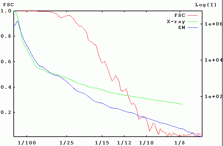
EM : 1D power spectrum of EM volume.
X-ray : Low-angle of X-ray scattering data, out to 8 Å.
FSC : Fourier shell correlation of the EM volume. The Fourier amplitudes need only be corrected out to the spatial frequency corresponding to the 0.5 FSC level, here 1/14 Å.

  • The EM Fourier amplitudes should be increased up to the level of the X-ray amplitudes.

  • To do this, create an enhancement curve from the EM and X-ray data. The enhancement curve is the factor by which the EM power spectrum curve must be multiplied so that it will approximate the X-ray curve.

  • Next, apply the enhancement curve as a filter to the EM volume.
  • The above data were plotted with a gnuplot script. The EM data were first multiplied to be in the same numerical range as the X-ray data (right axis), by running the procedure b06.pww.


    X-ray data

    Experimental X-ray curve, smoothed by Dmitri Svergun:
  • scattering8.tst exp. curve out to 8 Å
  • scattering11.tst exp. curve out to 11 Å

    These data are in the form of SPIDER document files with 4 columns:
    Frequency (1/Å)intensity multiplied by 60 (unknown)frequency in units of 2.93 Å


    Amplitude correction

    Step 1 : Create an enhancement curve

    Compute an enhancement curve, by comparing a 1D rotationally averaged power spectrum of the input volume to the X-ray spectrum. This curve represents the correction that must be applied to the volume's power spectrum in order to bring it up to the X-ray curve.
    enhance.bat
    Inputs: volume to be enhanced,
    X-ray scattering data
    Outputs: 1D power spectrum from volume,
    enhancement curve
    pwsc.bat procedure called by enhance.bat
         Given in input spatial frequency (Å), returns the corresponding intensity from the X-ray data.


    Step 2 : Fit a polynomial to the enhancement curve

    The fit command in gnuplot can be used to fit a curve to the enhancement function.
  • Input: the enhancement curve created by enhance.bat
  • Output: Fitting parameters A,B (and maybe C)
     gnuplot> K(x)=A*x*x+B
    
     gnuplot> fit K(x) 'fen.dat' using 1:3 via A,B
    
     gnuplot> plot 'fen.dat' using 1:3 with lines, K(x)
     A               = 623.42           +/- 20.02        (3.212%)
     B               = 13769.2          +/- 1.153e+04    (83.72%)
    
    Or, you can try a 3 parameter expression for a better fit:
     gnuplot> K(x)=C*x*x*x+A*x*x+B                              
     gnuplot> fit K(x) 'fen.dat' using 1:3 via A,B,C   
    
    Gnuplot script to save parameters to a file, and plot the curves in a gnuplot window.
    Gnuplot script to send output to a postscript file.


    Step 3 : Apply the enhancement parameters to the volume

  • Output: Filtered volume with corrected higher frequencies.

    applyabc.bat using the parameters obtained above, apply the enhancement/correction to the volume, then filter the volume at the resolution level.

    applyfen.bat Alternatively, apply the enhancement curve directly to the volume.


  • Updated Feb. 20, 2003