Three Dimensional Reconstruction of Single Particle Specimens using Reference Projections Without Defocus Groups
|
|
Three Dimensional Reconstruction of Single Particle Specimens using Reference Projections Without Defocus Groups |
|
Introduction |
In this protocol, CTF-correction is applied at the level of windowed particle images. In principle, though not yet implemented, astigmatic images can be corrected for. Lastly, interoperability with other software packages, which also correct for the CTF at the level of particle images is straightforward. However, we find that reconstructions sometimes show artifacts when using iterative backprojection methods (such as 'BP RP' or 'BP CG') thus these backprojection methods may be less usefull with CTF corrected images. <
Contents |
Links to further information |
Running SPIDER procedure files |
spider spi/dat @proc spi is the procedure file extension,
dat is the project data file extension, and
proc.spi is the procedure file.
Quick-start guideThis is a brief listing of steps in this protocol. For simplicity, options have been limited. For further information, see below. A procedure for testing a complete reconstruction using the Nature Protocols paper data set is provided. Data extension is assumed to be: |
In your working directory (e.g.user):
- cp $SPIDER_DIR/docs/techs/recon1a/spiproject.tar.gz .
- tar -xvf spiproject.tar.gz
- cd myproject
In your project directory (myproject):
- cp `which spider` ./spider
- Data loading choices:
- mv /actual-location-of-your/micrographs/raw* Micrographs/
spider spi/dat @make-params
spider spi/dat @resizevol
- tar -xvf $SPIDER_DIR/docs/techs/recon1a/natproc_data_mics.tar.gz
- (Due to its large size you may have to download this from Zenodo instead!!!)
- spider spi/dat @make-mic-list
- spider spi/dat @shrink-mic
- montagefromdoc ../sel_micrograph.dat sm_mic_* &
- spider spi/dat @ctffind
- montagefromdoc ../sel_micrograph.dat power/pw_avg*
- ctfmatch power/ctf* &
- spider spi/dat @make-ctf-cor
- spider spi/dat @make-noise-img
- Particle picking choices
- spider spi/dat @pick-at
- spider spi/dat @pick-lfc
- montagefromdoc win/sel_part_0001.dat win/winser_0001.dat &
- [Optional] Initial verification
- spider spi/dat @denoise-imgs
- Use Montage operation in
WEB.
- spider spi/dat @number-parts
- spider spi/dat @restack-n-ctf
- spider spi/dat @make-ref-views
- Alignment choices
- ./spider spi/dat @align
- ./spider spi/dat @pub-align
- spider spi/dat @select-byview
- spider spi/dat @avg-filter-byview
- spider spi/dat @plot-cc-vs-view
- spider spi/dat @show-ref-views
- [Optional] Classification-based verification
- spider spi/dat @verify-class-byview
- verifybyview views/prj001
- spider spi/dat @verify-combine-classes
- spider spi/dat @plot-cc-vs-view
- spider spi/dat @show-ref-views
- spider spi/dat @plot-ref-views
- spider spi/dat @parts-vs-defocus
- spider spi/dat @best-imgs
- spider spi/dat @recon-regroup
- Reconstruction choices
- ./spider spi/dat @recon
- ./spider spi/dat @pub-recon
- spider spi/dat @plot-fsc-curve
- Refinement choices
- ./spider spi/dat @refine
- ./spider spi/dat @pub-refine
- spider spi/dat @plot-fsc-curves
Creating a new reconstruction projectAt the start of a reconstruction project, a project directory has to be set up with the proper subdirectories and procedure files. Run these procedures in the project/ directory. |
Create a project directory containing the required subdirectories and procedure files
tar zxvf $SPIDER_DIR/docs/techs/recon1a/spiproject.tar.gz mv myproject ribosome
Create a parameter document file
Some processing information is stored in a project-wide document file that is used by many procedure files. Run the interactive procedure: make-params.spi in the top directory of your project. It creates a document file:| ¤ | params: | SPIDER document file containing the reconstruction parameters. |
[Optional] Resize reference volume
A reference volume, named: ref_vol, is required in the myproject directory. If the pixel size of your reference volume (key 5 in the params file) and/or the dimensions (key 17 in params) do not match the data that you will be processing, then run: resizevol.spi which reads: orig_reference_volume, from the top-level project directory to resize the volume. This creates:| ¤ | ref_vol: | Resized reference volume. |
Copy your current spider executable into your project
cp `which spider` ./spider Preparing micrographsPlace digitized micrographs in the Micrographs/ directory. Run these procedures in the Micrographs/ directory. |
It reads filenames and ###.frames.mrc (Where ### denotes stem name of input set). It creates:
| ¤ | ###: | SPIDER micrograph stacks. |
| ¤ | filtstk_###: | Filtered micrograph stacks. |
| ¤ | shift_doc_###: | Raw alignment shift doc file. |
| ¤ | mlr_shift_doc_###: | Refined alignment shift doc file. |
| ¤ | shstk_###: | Aligned frame image stacks. |
| ¤ | ali_###: | Summed aligned image. |
mv /actual-location-of-micrographs/*###* Micrographs/
The procedures below can accept SPIDER, Hiscan TIFF, PerkinElmer, ZI, and Nikon Coolscan data. These files may have been compressed with gzip, if so be sure to indicate compression in the params file.
tar -xvf $SPIDER_DIR/docs/techs/recon1a/natproc_data_mics.tar.gz | ¤ | sel_micrograph: | Micrograph selection doc file listing 4 micrographs used later in the protocol. |
| ¤ | Micrographs/raw****: | Four micrograph images. |
| ¤ | orig_reference_volume.dat: | Reference volume. |
| ¤ | reference_volume.dat: | Reference volume. |
| ¤ | params: | Reconstruction parameter file. |
Selecting micrographsGenerate a list of micrographs and screen the micrographs. Run these procedures in the Micrographs/ directory. |
Create a selection file for micrograph file numbers
| ¤ | sel_micrograph: | Micrograph selection doc file listing the numbers of the micrograph files to be processed. |
mkfilenums.py ../sel_micrograph.dat Micrographs/raw*
[Optional] Shrink micrographs
Before screening the micrographs for quality, it may be helpful to shrink the micrographs in order to quickly scan through them.| ¤ | sm-mic****: | Reduced size micrographs. |
[Optional] Screen micrographs
Screen the micrographs using the Python script: montagefromdoc.py. The syntax, not including the proper data extension is:montagefromdoc ../sel_micrograph.dat sm-mic* | ¤ | ../sel_micrograph: | An updated micrograph selection file. |
Contrast Transfer Function Parameter EstimationEstimate defocus of each micrograph by calculating its power spectrum. For more information, see:
Run these procedures in the Power_Spectra/ directory. |
Calculate the power spectrum for each micrograph and determine CTF defocus values:
ctffind.spi (which calls SPIDER procedure load-mic.spi) reads each micrograph, computes an averaged power spectrum, and estimates defocus, astigmatism, and cut-off frequency using SPIDER operation: 'CTF FIND'. This operation invokes the functionality from the MRC ctffind3 software. This operation reads: ../params, ../sel_micrograph, and ../Micrographs/raw****. It creates:| ¤ | power/pw_avg_****: | 2D power spectra, each is an average of many smaller power spectra calculated over the surface of the micrograph. |
| ¤ | power/diag_pw_avg_****: | 2D diagnostic power spectra, which likewise is an average of smaller power spectra calculated over the surface of the micrograph. |
| ¤ | power/roo_****: | Rotationally averaged power spectra. |
| ¤ | power/roo_doc_****: | Doc files containing 1D profiles of the rotationally averaged power spectra. These doc files can be plotted with gnuplot or pyplot |
| ¤ | defocus: | A doc file of CTF defocus values. |
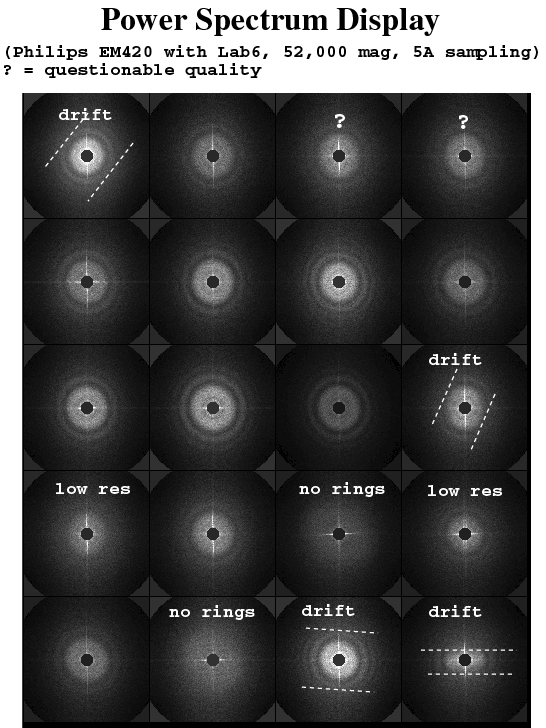
Check the Thon rings in the power spectrum images
The power spectra are equivalent to diffraction patterns obtained in an optical diffractometer. It is absolutely important that you screen the spectra before proceeding any further.
| Things to look for: Are the Thon rings round? Do the rings extend to high resolution? You can discard micrographs that show one of the following artifacts: Rings that are cut off unidirectionally (evidence of drift). Rings that are elliptical, or even hyperbolic (evidence of astigmatism). |
 |
The power spectra can be examined using three methods:
Look at the power spectra: power/pw_avg_**** in a WEB montage (using size reduction).
More informatively, look at the diagnostic power spectra: power/diag_pw_avg_**** in a WEB montage (using size reduction).
The CTF for each micrograph can be examined by using
ctfinfo.spi (which uses SPIDER operation:
'TF ED').
It reads:
../params and power/pw_avg_****.
It creates:
| ¤ | power/ctf_****: | Doc file containing CTF curve and noise info for each micrograph. |
montagefromdoc ../sel_micrograph.dat power/pw_avg_*.
Use the GUI to select/reject desired micrographs.
Generate CTF profiles and correction files for each micrograph.
make-ctf-cor.spi generates sets of CTF files and 1D CTF profiles. The CTF correction files will be applied to subsequent particle images. The procedure reads: ../params, defocus, and optionally: power/roo_doc_****. It creates:| ¤ | power/flipctf_****: | Phase flipping CTF correction files. |
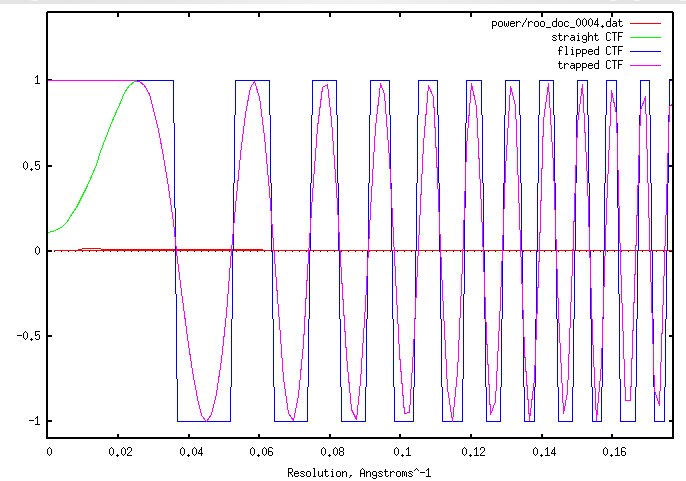
| ¤ | power/flipctf_doc_****: | Optional doc file containing 1D profiles of straight CTF, phase-flipped CTF, CTF with unaffected low-resolution terms, etc. |
| ¤ | viewtrap.gnu: | Optional Gnuplot script for plotting the 1D profiles of the the computed transfer functions. |
|
In the Gnuplot output script viewtrap.gnu one micrograph is chosen to plot the corresponding 1D transfer-function profiles. By default, the micrograph with the highest defocus is chosen. To plot a different micrograph's profiles, set the parameter [mic2plot] to a different micrograph number in make-ctf-cor.spi, or simply edit the Gnuplot script. The plot should be displayed automatically, if not click here. The 1D profile outputs are interchangeable for CTF correction in the later procedures, but by default the power/flipctf_**** files will be used. |
Particle Windowing and Initial VerificationA particle picking procedure file analyzes each micrograph, cutting out small windows of likely particle candidates. This is followed by a manual selection process that identifies the good particle images and rejects the bad ones. Particles automatically output by the procedure file are said to be windowed; the subset that are manually chosen are said to be verified. Run these procedures in the Particles/ directory. |
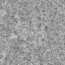
Select a background noise file
A noise image is required to normalize the backgrounds of the particle images during automatic particle picking. Do one of the following:| ¤ | noise: | A noise image. |
|
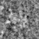
This noise file has been randomly selected from a set of files (tmpnoise/noi***) that are windowed from regions in the micrograph that appear not to contain any particles. View the selected noise file. If the image contains any structure such as a particle or junk then select one of the other candidates and copy it to noise.dat. |
 Noise image |
Run automatic phase of particle selection
Any of the following three approaches can be used.| ¤ | win/sel_part_****: | Particle selection doc file for each micrograph. |
| ¤ | win/data_bymic_****: | Stacked particle images. |
| ¤ | coords/pkcoor****: | Peak coordinates for particles. |
| ¤ | coords/ulcoor****: | Upper-left corner coordinates for particle windows. |
| ¤ | win/sel_part_****: | Particle selection doc file for each micrograph. |
| ¤ | win/data_bymic_****: | Stacks of particle images for each micrograph. |
| ¤ | coords/pkcoor****: | Peak coordinates for particles. |
| ¤ | win/sel_part_****: | Particle selection doc file for each micrograph. |
| ¤ | coords/pkcoor_****: | Pixel coordinates for center of particle images. |
| ¤ | win/data_bymic_****: | Stacks of particle images for each micrograph. |
[Optional] Low-pass filter particle images before particle verification.
Visual selection of good particles (the optional next step) is easier if
the particles have been low-pass filtered beforehand.
denoise-imgs.spi
filters a set of images, adjusting filter settings for each micrograph,
based on its defocus. It reads:
../sel_micrograph and
win/data_bymic_**** .
It creates:
| ¤ | filt/data_bymic_****: | Stacks of low-pass filtered particle images. |
|
Use the filtered particles, not the raw particles, during visual selection. |
 Unfiltered |
 Filtered |
[Optional] Verify the windowed particles
This step is optional if using classification-based verification later on. Sort through the windowed particle files to eliminate any non-particles using one of these methods:
montagefromdoc win/sel_part_1234.dat filt/data_bymic_1234.dat | ¤ | win/sel_good_****: | Particle selection doc files, one for each micrograph. |
Remove duplicate particles, and assign a unique global particle number for each image
number-parts.spi will assign a global particle number that will help track particles later as they are grouped and regrouped. This number will optionally be placed in the particle image file's header for future reference. Also created new selection files for unduplicated 'good' images.
It reads: sel_micrograph, and win/data_bymic_****.If you know from experience that pick-lfc.spi, for example, windows too many particles, you can set the register [max-particles] to the expected number. The first [max-particles] number of particles will be retained, assuming that the particles are sorted from best to worst, as is the case in pick-lfc.spi.
If you are appending to an existing data set, set the register [first-global] to a number unused prior, for example, the last particle number used plus 1.
This procedure will optionally add the global particle number to the image header, specified with the variable [labelheader-yn]. As particle images get copied from one place to another -- e.g., micrograph stacks, parallelization stacks, etc. -- this identifier will be retained in the copies. Modification of the image stacks in this manner is somewhat slow, in my test case taking several minutes instead of less than one minute. However, if time is not an issue, or if you anticipate bookkeeping issues, keep this header-assignment step, which is active by default.
The procedure creates:| ¤ | good/sel_part_****: | A set of particle selection doc files, one for each micrograph, listing unduplicated selected particle numbers. |
| ¤ | win/micwin2glonum_****: | A set of look-up tables for the selected particles in each micrograph, mapped to a unique global particle number. |
| ¤ | win/glonum2micwin: | A reverse look-up table for the selected particles in each micrograph, mapped to a unique global particle number. |
| ¤ | percent_selected: | A doc file listing percentages of automatically picked vs manually selected particles for each micrograph and overall. |
AlignmentReference images are generated from the reference volume. Data particles are compared to each reference to find the best match, and the corresponding transformations (shifts and rotations) are written to a doc file. Finally, the transformations are applied to the data images, aligning them to the references. Run these procedures in the Reconstruction/ directory. |
nedit recon-settings.spi | ¤ | [num-grps]: | Number of computational groups. |
| ¤ | [shrange]: | Translation search range. |
| ¤ | [step]: | Translation step size. The operation
'AP SHC'
tries different combinations of shifts in increments of [step]
up to [shrange], performs an orientational alignment,
and chooses the best one. (See notes in the
'AP SHC' documentation.) For example, with a [step] and [shrange] both of 2, 'AP SHC' will try shifts of (-2,2),(0,2),(2,2),(-2,0),(0,0), (2,0),(-2,-2),(0,-2), and (2,-2). |
| ¤ | [r2]: | Outer alignment radius (pixels). The sum of [shrange] and [r2] must be less than half the image dimension. |
| ¤ | [incore-yn]: | Will load input images into incore stack. This more efficient, but if you have insufficient memory, set it to zero. |
In the following file names [win_dir] denotes a directory used mainly for stacked windowed particle images and [rec_dir] denotes a directory used mainly for alignment and reconstruction output. This allows for easy repetition of runs with differing parameter settings and minimizes moving/duplication of files. In the following we will assume that you have set: [win_dir] = '../win_0' and [rec_dir] = '../rec_0'.
CTF correct images and assign to groups for parallelization.
stackwins-n-ctf.spi restacks particles listed in a set of particle selection files into the number of stacks specified in: recon-settings.spi. If alignment is not going to be parallelized the number of new groups can be set to 1 (though not required).| ¤ | [win_dir]/sel_group: | New group selection doc file. |
| ¤ | [win_dir]/sel_part_***: | New particle selection doc files. |
| ¤ | [win_dir]/data_***: | New particle image stacks. |
| ¤ | [win_dir]/part2glonum_***: | Lookup tables listing global number for particles. |
Create reference projections for alignment from a reference volume
Reference projections (images) are views of the reference volume at known angles. In what follows, angular sampling is set to 15 degrees, which results in 83 reference projections. A reference volume from the top level project directory is needed to create the projections. The row and column dimensions of the reference volume must match the dimensions of the particle windows. (see resizevol.spi)
make-ref-views.spi reads: [win_dir]/ref_vol. It creates three files:| ¤ | [rec_dir]/sel_proj: | List of reference views. |
| ¤ | [rec_dir]/ref_angs_00: | A doc file from 'VO EA' listing the three Euler angles for each of the projections. |
| ¤ | [rec_dir]/ref_projs_00: | Stacked reference images created using: 'PJ 3Q' corresponding to the angles in the preceeding file. |
Align particles to the reference projections
Alignment is compute-intensive and benefits by parallelization.
The following alignment choices depend on whether using you are using
PBS for parallelization
on a compute cluster or are running the alignment serially without a cluster.
spider spi/dat @align spider spi/dat @pub-align 1 & Both options read: [win_dir]/ref_vol , [rec_dir]/ref_projs_00, and [rec_dir]/ref_angs_00 . They create:
| ¤ | [rec_dir]/dala_01_***: | Aligned stacks of particle images for each group. |
| ¤ | [rec_dir]/align_01_***: | Shift and rotation parameters for each group. |
| ¤ | [rec_dir]/align_01: | Consolidated shift and rotation parameters for all groups. |
Compute Averages and Verify ParticlesFor all projections, all aligned particles of a given reference view are averaged together. Further particle selection is made by selecting a correlation cutoff threshold to reject some particles. The distribution of particles among projections can be displayed. Run these procedures in the Averages/ directory. Note: *** denotes image group, ### denotes view, ??? denotes class |
nedit verify-settings.spi Make particle selection doc files listing particles corresponding to each reference projection
select-byview.spi (which calls: verify-settings.spi) reads: [win_dir]/sel_group , [win_dir]/sel_part_*** , [rec_dir]/ref_angs_01_***, and [rec_dir]/align_01_*** . It creates:| ¤ | views/prj###/sel_part_byv: | List of particles associated with each reference view |
| ¤ | views/parts_vsview_all: | Summary of number of particles associated with each reference view. |
[Optional] Create average images for all projection views and, optionally, write out filtered, aligned images. This step is required if using the classification-based verification.
To skip the output of the filtered images, set the register [save-filt-yn] in the procedure parameters to: 0. These filtered images are required if using classification-based verification. The setting for: [reduction] is to save processing time and disk space.
avg-filt-byview.spi reads: [win_dir]sel_proj , [rec_dir]/dala_01_*** , and views/prj###/sel_part_byv. It creates:| ¤ | views/prj###/allavg: | Stacks of average images for each set of projections. |
| ¤ | views/prj###/filtavg: | Filtered, aligned image stack [Optional, required for classification-based verification] |
montagefromdoc sd_vsview_all.dat prj***/allavg The next two steps help to identify a threshold correlation coefficient that describes true particles as opposed to any erroneously selected particles.
Create histograms of the number of particles vs. the cross correlation value
plot-cc-vs-view.spi reads:
[rec_dir]/sel_proj and
views/prj###/sel_part_byv.
and creates a histogram that plots the number of particles vs. the cross correlation
value. Experiment with the parameter [num-bins] if
you want finer sampling per bin, or coarser (and thus more particles per bin).
The procedure creates:
| ¤ | prj###/sel_part_combined: | Combined doc file of the same format as views/prj###/sel_part_byv. |
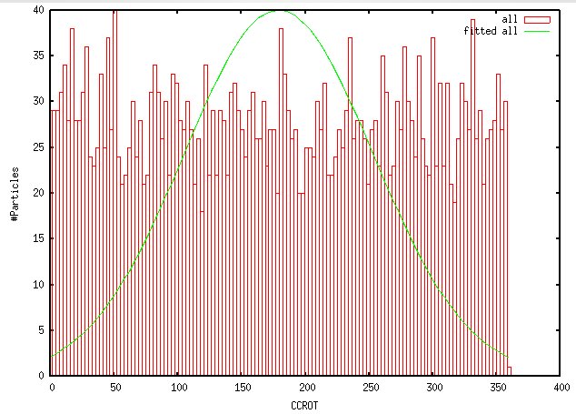
| ¤ | cc_vsview_all: | Histogram doc file of cross correlation values. |
| ¤ | cc_vsview_all.gnu: | Gnuplot script for plotting the correlation histogram. |
|
The output Gnuplot script cc_vsview_all.gnu will overlay the correlation histogram of the particle images with a Gaussian profile. If the histograms display a bimodal distribution, the higher peak may correspond to actual particles, while the lower peak may show noise. A threshold can be chosen between two such peaks. The plot should be displayed automatically, if not click here. |
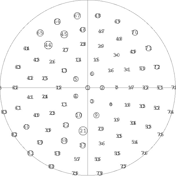
[Optional] Check the spatial distribution of views (angular directions) for the reconstruction
plot-ref-views.spi reads
views/parts_vsview_all.
It creates script files of gnuplot commands:
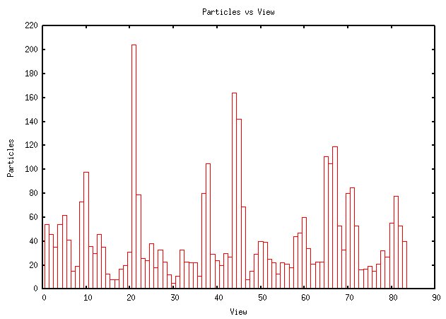
| ¤ | parts_vsview_all.gnu | Gnuplot script to plot a histogram of number of particles vs projection view. |
|
The output Gnuplot script parts_vsview_all.gnu will plot a histogram of number of particles vs projection view. The plot should be displayed automatically, if not click here. |
| ¤ | show_ref_views: | SPIDER image showing distribution of sample images among the various reference projections. |
[Optional] Classification-based verification
Further information is provided at the classification-based verification page. Briefly, this sub-protocol reads: views/prj###/sel_part_byv and views/prj###/filtavg and classifies the particles corresponding to each reference projection.
Summary of required steps:| ¤ | verify-class-byview.spi: | Classifies the particles corresponding to each reference projection. |
| ¤ | verifybyview.py | Select particles by orientation and classification: after separation. |
| ¤ | verify-combine-classes.spi: | Collects information about selected particles. |
| ¤ | plot-cc-vs-view.spi: | Creates histogram of cross correlation values. |
| ¤ | parts-vs-defocus.spi: | Creates histogram of particle numbers vs defocus values. |
If performing this verification step, remember to alter the input file selection in: best-imgs.spi.
Create new group and particle selection files and [optionally] limit over-represented angular projections
Run this procedure even if you aren't limiting over-represented views as downstream procedures will need the outputs.
best-imgs.spi optionally limits the numbers of images per reference view direction as specified by parameter: [maxim]. This will limit over-represented angular projections which may cause a shape error in the reconstruction. If you do not wish to limit over-represented views, set the parameter: [maxim] to -1 (the default).
Set the parameter: [use-particles] to indicate whether you want to use the particle selection files from images without classification-based verification, "good" images from classification-based verification, or "rechecked good" images from classification-based verification.
This parameter will choose between reading: views/prj???/sel_part_byv_good , or views/prj???/sel_part_byv_goodB , (from verify-recheck.spi) in place of: views/prj???/sel_part_byv_sort .
best-imgs.spi then reads:
[rec_dir]/sel_proj ,
[rec_dir]/sel_group , and
[rec_dir]/sel_part_sort_*** .
It creates:
| ¤ | sel_group_best | Group selection file |
| ¤ | sel_part_best_*** | List of particles selected for each new group |
| ¤ | views/prj###/sel_part_byv_best | List of particles retained from each reference view |
| ¤ | part_vsview_best | Summary of number of images in each reference view. |
3D ReconstructionUse the selected aligned particles to create an initial 3D volume. To estimate the nominal resolution of the resulting structure, the particle images are split into two equal sets, and the two resulting reconstruction volumes are compared. Run these procedures in the Reconstruction/ directory. |
nedit recon-settings.spi | ¤ | [bp-type]: | Backprojection method. More information below. |
| ¤ | [stk-opt]: | Stack options (e.g., 0 to read from original location, 1 to copy into RAM, or 2 to copy temporarily to disk). |
For the parameter [bp-type], the Fourier-based backprojections -- 'BP 32F' (option 2 in bp-settings.spi) or 'BP 3N' (option 4) -- are recommended. The iterative, real-space methods -- 'BP RP' (option 3) or 'BP CG' (option 1) -- sometimes cause artifacts in the reconstruction. These artifacts include a rise in the FSC at high resolution, or sometimes ripples in the reconstruction when viewed as Z-slices. The artifacts may be due to inaccuracy in the estimated defocus. Feel free to experiment, but be wary of the output.
Assign particles into groups for 3D reconstruction
recon-regroup.spi offers the choice between grouping particles into new groups or keeping the old groups. If you have no desire to regroup the particles, set the parameter [num-stacks] to 0, which will simply create links to the existing files for downstream files to read. Among the reasons to regroup the particles could be that the number of particles may have changed since groups were first established -- for example following classification or limiting overrepresented views or by CC value -- or perhaps the number of compute nodes available has changed. It reads: ../Averages/sel_group_best_*** , ../Averages/sel_part_best_*** , [rec_dir]/data_*** , [rec_dir]/align_01_*** , and [rec_dir]/dala_01_*** . To perform a dry run -- for example to see how big the groups will be -- set the parameter [stacks-yn] to 0.
recon-regroup.spi creates:| ¤ | [win_dir]/sel_group: | Group selection document file. |
| ¤ | [win_dir]/sel_part_***: | Doc file listing the particles in each group. |
| ¤ | [win_dir]/data_ctfd_***: | Stack files containing particle images for each group. |
| ¤ | [win_dir]/dala_01_***: | Stack files containing particle images for each group. |
Compute 3D reconstruction
Create paired reconstructions for each group, merge group reconstuctions into final combined reconstruction, and compute reconstruction resolution. The following options will depend on whether using you are using a PBS cluster or are running the reconstruction serially without a cluster.
spider spi/dat @recon spider spi/dat @pub-recon 1 & | ¤ | sel_part_01_***_s1: | List of odd numbered images for each group. |
| ¤ | sel_part_01***_s2: | List of even numbered images for each group. |
| ¤ | vol_01_***_s1: | Reconstructed volume from first subset of images for each group. |
| ¤ | vol_01_***_s2: | Reconstructed volume from second subset of images for each group. |
| ¤ | vol_01_***: | Combined reconstructed volume for each group. |
| ¤ | vol_01: | A 3D reconstruction from entire set of particles. |
| ¤ | fsc_doc_u: | Doc file containing unmasked FSC curve for final reconstruction. |
| ¤ | fsc_doc_m: | Doc file containing masked FSC curve for final reconstruction. |
| ¤ | resolution: | Doc file containing masked and unmasked resolution (in Angstroms). |
    recon
    recon-settings

    recon
    merge-fsc-filt
|
pub-recon recon-settings recon-loop merge-fsc-filt |
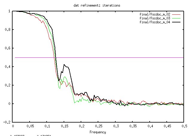
Check the FSC curve by viewing a plot.
plot-fsc-curve reads: fsc_doc_m . It creates a text file of gnuplot commands:| ¤ | fsc.gnu: | Gnuplot script for plotting the resolution curve. |
|
The output Gnuplot script fsc.gnu will plot the fsc curve and should be displayed automatically, if not click here. Examine this plot and see if there is an unusual curve. |
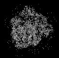
View the filtered volume
This reconstruction vol_01 is known as the initial volume. View the filtered volume as a surface by using the Surface operation in WEB or by loading the volume in Chimera.
|
View the volume as slices using the Montage operation in
WEB or in
montage.
|
RefinementRefinement essentially performs the reconstruction steps repeatedly, decreasing the angular resolution of reference projections with each iteration, thereby giving the data particles a chance to find a better approximating reference match each time. The data particles are allowed to "settle in" and find better fitting angles, than the initial choices. Refinement is a computationally expensive operation. Before starting a refinement, check the results of the above reconstructions, to ensure that the initial volume is reasonable to start. Refinement is currently set to re-start with the unaligned images instead of the alignments from the reconstruction step, since this does not take much additional time at coarse reference angles. The workflow is set up to create two subset reconstructions as needed for 'gold standard' resolution determination. Run these procedures in the Refinement/ directory. |
Access your refinement directory, e.g.:
cd /mydir/project/Refinement
Remove existing output files currently in refinement directory, e.g.:
rm -f  results.*
    LOG.*  fort.* work/*   core*
Copy latest SPIDER executable into the current directory and rename it: spider.
This ensures that same SPIDER executable is used throughout whole refinement, e.g.:
cp /usr/local/spider/bin/spider_linux_mp_opt64.22.17 spider
Edit refine-settings.spi to set
necessary values for refinement parameters and check input file names,
e.g.:
nedit refine-settings.spi
The following files are needed, where
'[win_dir]' denotes input directory,
'[refi_dir]' denotes refinement output directory,
'***' denotes group number, and
'##' denotes iteration number:
| ../ref_vol: | Reference volume. (one) |
| [win_dir]/sel_group: | Group selection file. (one) |
| [win_dir]/sel_part_***: | Particle selection files. (one / group) |
| [win_dir]/data_***: | Unaligned, CTF corrected, stacked image files. (one / group) |
| [win_dir]/scattering: | Optional X-ray scattering power spectrum file. (one) |
| [win_dir]/mask: | Optional amplitude enhancement mask file created from outer contour. (one) |
spider spi/dat @refine 0 &
ssh gyan
./spider spi/dat @pub-refine 0 &
where 0 will be the number of the top-level SPIDER results file.killspi to stop any remaining parallel jobs that
belong to you. wherespi to find any remaining parallel jobs. If any
remain, use killspi again until they are all gone.
rm -rf results.* LOG.* work/ local/ final/ core* fort.*
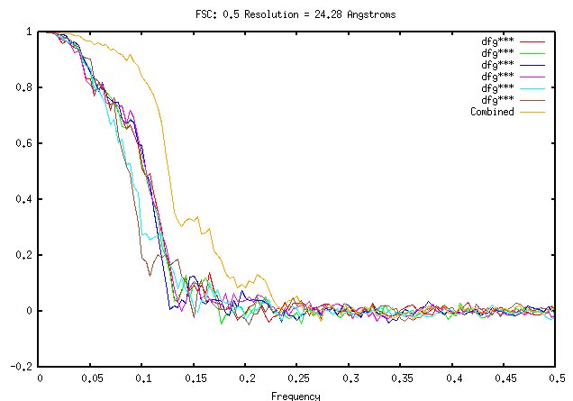
Plot the refinement resolution curves
plot-fsc-curves.spi reads:
[refi_dir]/fscdoc_m_##.
It creates a gnuplot script:
| ¤ | [refi_dir]/fsc_iter.gnu: | Plots FSC resolution curve for each iteration of refinement. |
refine .. refine-settings .. show-r2.spi .. refine-setrefangles.spi .. pub-prjrefs .. refine-loop .. refine-smangloop .. refine-bp .. merge-fsc-filt .. enhance |
pub-refine .. refine-settings .. show-r2.spi .. refine-setrefangles.spi .. pub-prjrefs .... pub-submit ...... memforqsub.spi ...... qsub.pbs ...... pub-refine-start ([task]=2) ........ refine-settings ........ refine-prjloop .. pub-submit .... memforqsub.spi .... qsub.pbs .... pub-refine-start ([task]=0/1) ...... refine-settings ...... refine-loop ...... refine-smangloop ........ refine-bp .. merge-fsc-filt .... enhance pub-refine-fix |
| 'VO EA' | Create reference angles for this iteration |
| 'PJ 3Q' | Create stack holding reference projections. |
| 'CP' | Copy current unaligned images to inline stack for speed |
| 'AP REF' or 'AP SHC' |
Find reference projection that matches each current aligned image. Find alignment parameters to match selected reference projection. |
| 'RT SF' | Rotate, mirror, and shift unaligned original image to create current aligned image |
| 'BP 3F' or 'BP CG' | Calculate refined group volume from new aligned images and angle data |
| FSC | Calculate phase residual for refined group volume |
| 'AS S' | Merge refined group volumes |
| 'AS S' | Merge first sub-set refined group volumes |
| 'AS S' | Merge second sub-set refined group volumes |
| 'FSC' | Calculate resolution for combined volume |
| enhance.spi | Optional amplitude enhancement |
| 'FQ' | Filter final corrected volume to limit resolution |
| ¤ | [refi_dir]/vol_##_s@_raw: | Unfiltered subset volumes (two / iter) |
| ¤ | [refi_dir]/vol_##_s@_unfilt: | Unfiltered, deconvolved subset volumes (two / iter) |
| ¤ | [refi_dir]/vol_##_s@: | Filtered, deconvolved subset volumes (two / iter) |
| ¤ | [refi_dir]/vol_##_unfilt : | Complete unfiltered volume (one / iter) |
| ¤ | [refi_dir]/vol_## : | Complete filtered volume (one / iter) |
| ¤ | [refi_dir]/vol_##_cent: | Complete filtered, centered volumes (one / iter) |
| ¤ | [refi_dir]/fscdoc_m_## | Masked FSC resolution curve doc files (one / iter) |
| ¤ | [refi_dir]/resolutions: | Doc file listing resolution at each iteration. (one) |
| ¤ | [refi_dir]/align_##_***_s@: | Alignment parameter doc files (two / group / iter) |
| Proj. angle - PSI | Proj. angle - THETA | Proj. angle - PHI | Reference # | Image # | Inplane rotation angle | X Shift | Y Shift | Number of proj. | Angular difference | CC Rotation | Current Inplane angle | Current X Shift | Current Y Shift | Mirror & Cross corr. |
Other Useful Methods |
References |
Modifications logFor a more complete list of changes, see individual procedures. |